Post-hoc tests and determining where differences occur

When you run a t-test or Mann Whitney test, a significant difference (p < 0.05) means that the sample means (or medians) are significantly different from each other. The larger average is significantly bigger than the smaller average. So, obtaining the means (or medians) for each category (as you probably did when initially exploring the data) will tell you what you need to know.

However, when you run an ANOVA or Kruskal Wallis test, your p values only tells you there is a difference somewhere between the means (or medians). As an example, if we had three categories a, b and c; then a significant difference in an ANOVA may mean:

a is significantly bigger than b, b is significantly bigger than c

a is significantly bigger than b, b is not significantly different to c

a is not significantly different to b, b is significantly bigger than c

or a number of other possible combinations.

To determine where the differences occur, we run something called a post-hoc test, following the ANOVA.

While it is also possible to run a post-hoc test following a Kruskal Wallis test, this can not be done in SPSS, and requires some more advanced R skills to do this. The video on the comparing means page does explain how to do this, but it may be easiest to ask for more help on this in a drop in session.

An alternative to a post-hoc test would be to make a graph of means and 95% confidence intervals, as described last year, and look for overlap between the confidence intervals. However, a post-hoc test is probably more reliable than this method.

The videos on the comparing means page guide you through this process step by step too. But as a quick reference:

In SPSS:

Check the ANOVA output - was there a significant difference in the ANOVA - if not, do not run post-hoc tests.

Analyse -> Compare means -> One Way ANOVA

This time, select PostHoc

Tick the SNK or the TUKEY box

Run the ANOVA again

In R:

Check the ANOVA output - was there a significant difference in the ANOVA - if not, do not run post-hoc tests.

run the command: TukeyHSD(analysis1, 'independent')

Here 'analysis1' is whatever name you have given the the ANOVA, and refers to the information stored in this variable.

Replace 'independent' with the name of the independent variable - but for some reason, this time, the name needs to be in inverted commas or quotation marks

Examining and interpreting the output

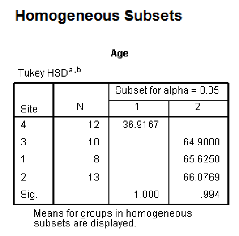
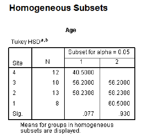
A typical post-hoc test output from SPSS produces a LOT of output. The most useful output looks like one of the following three boxes:

This example is fairly easy to interpret. The values are the means for each of the different categories. Site 4 is in a different column to the other sites. So it can be concluded that site 4 is significantly different to the other sites.

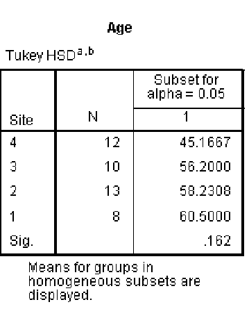
This example is even more complex to interpret. The values are the means for each of the different categories. All sites are in the same column - so the Tukey test assumes all sites are not significantly different from each other. However, if you have already found a significant difference using ANOVA, then the correct interpretation of this is that the site with the lowest mean (site 4) is significantly different to the site with the highest mean (site 1). We can not determine any other differences between sites.

This example is more complex to interpret. The correct interpretation of this is that the site with the lowest mean (site 4) is significantly different to the site with the highest mean (site 1). We can not determine any other differences between sites, as site 1 is in the same column as 2 and 3. However, site 4 is also in the same column as 2 and 3.

From R you get simpler output which looks like this:

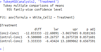
While these are different data to the SPSS example, R makes a list of each comparison that is possible, and specifies a p value for each one.

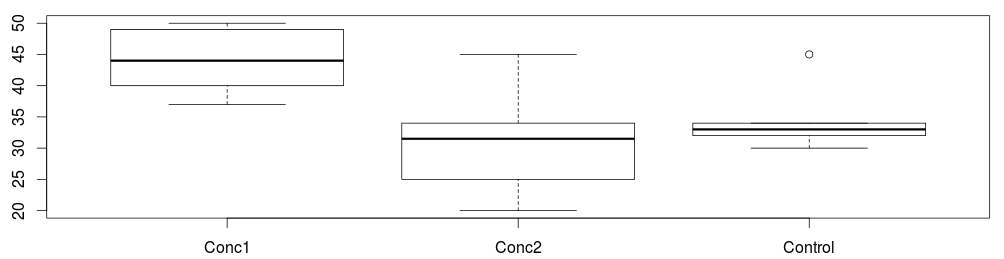
Here you can see that Concentration 1 and Concentration 2 are significantly different. No other comparisons are significant, although Concentration 1 and Control has a p value of 0.057, this is above 0.05, so is not classed as significant.

Reporting results in a report, paper or assignment

DO NOT copy and paste output of SPSS or R into your work - unless you are specifically asked to put it in an appendix.

In some cases, you may be able to explain these results in a simple line of text. For example:

Subjects taking concentration 1 showed a significantly higher level of white blood cells than those taking concentration 2. However, neither concentration showed significantly different levels to the control treatment.

Also, it can be possible to include information on a figure, as in this example:

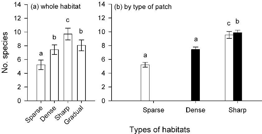
Figure 3. Effects of composition of experimental landscapes on numbers of species

Mean (±SE) numbers of species in experimental landscapes with different composition (Sparse, Dense, Sharp and Gradual). Numbers of species are averaged across 2 sites and 3 replicate experimental landscapes. In (b), bars with different patterns indicate numbers of species in different types of turfs in landscapes of different composition: sparse (clear), dense (solid) and intermediate (striped) turfs. Letters indicate significant differences between means (SNK at P<0.05; analyses in Table 2).

Figure from Matias et al. (2013)

In this case, bars labelled 'a' are not significantly different from each other. Where as bars labelled 'b' are different from those labelled 'a' and so on.

Back Next